2.1 Creating spaces: cost functions and matrices symmetry
all you need to know about how to write nice cost functions and how to make dispersal harder in specific directions
14.10.2026
Source:vignettes/b-cost-functions-mtx-symmetry.Rmd
b-cost-functions-mtx-symmetry.RmdIntroduction
In nature, species dispersal are often not symmetrical, i.e., it could be harder to follow some paths than others. For example, the topography of a region can be quite rugged, featuring areas of steep slopes. In this case, animal and plant dispersal may face resistance in directions of higher elevations, while descending is clearly less costly. Another example is river flow. Aquatic organisms may disperse more easily in the direction of the river flow instead against it. In these cases, when constructing distance matrices to simulate species dispersal, a asymmetrical matrix is necessary. This matrix will tell us (and gen3sis2) that moving from site A to site B () could have different cost than moving .
In gen3sis2 the symmetry of the distance matrices are straightforward controlled by the cost_function itself, which is highly customizable. In this vignette, we will see how to write many different forms of cost functions and how they impact the distance matrices.
Starting simple: a cost function anatomy
In gen3sis2, users can (and are encouraged to) construct a multitude of cost functions. It has a few rules: (1) it must follow R syntax; (2) it must return a single numerical value, or Inf; (3) the first two arguments must be source and dest; and (4) any other argument used must have a default value. To do that, gen3sis2 provides users with useful information about the source and the destination cells:
“index”: Raster cell index
“coordinates”: Cell centroid coordinates
“value”: Variable values in cell
“habitable”: Habitability in cell
All information is derived from the input raster used. Raster cell index is always an integer, and habitability is always boolean (TRUE or FALSE). They work as building blocks: users can organize and use them as wished. It is not mandatory to use all of them (or any, actually), but together they can produce very interesting dispersal rules, as we will see later.
In the previous vignette, we defined the following cost function:
cf <- function(source, dest) {
    if (!all(source$habitable, dest$habitable)) {
        return(2/1000)
    } else {
        return(1/1000)
    }
}
Note how that follows the rules cited above. Most importantly, note that to call source and destination cells habitability information the $ is used. This is because source and dest parameters will receive lists within the matrices calculations. For that reason, when manipulating cell information, R list syntax must be used.
To show how the cost functions deal with cells information, lets simulate two cells. Imagine the first two cells of a raster with temperature and air humidity information, that are in the same row and consecutive columns:
source <- list(index = 1, coordinates = c(x = 0, y = 0), value = c(temperature = 30,
    air_humidity = 40), habitable = TRUE)

dest <- list(index = 2, coordinates = c(x = 0, y = 1), value = c(temperature = 35,
    air_humidity = 25), habitable = TRUE)
Inside the cost function, all information can be accessed using simple list syntax, with $. To explore that, imagine that the cost will be defined by the temperature difference between the cells divided by the mean air humidity. In that case, we will write the cost function as:
cf <- function(source, dest) {
    temp_difference <- (source$value[["temperature"]] - dest$value[["temperature"]])
    mean_humidity <- (source$value[["air_humidity"]] + dest$value[["air_humidity"]])/2
    cost <- temp_difference/mean_humidity

    return(cost)
}

cf(source, dest)
#> [1] -0.1538462
Getting complex: adding an external information
One possibility to make more complex cost functions is to implement additional information or variables in it. To illustrate this, let’s add a “base_cost = 1”, to control cost values:
cf <- function(source, dest, base_cost = 1) {
    temp_difference <- (source$value[["temperature"]] - dest$value[["temperature"]])
    mean_humidity <- (source$value[["air_humidity"]] + dest$value[["air_humidity"]])/2
    cost <- temp_difference/mean_humidity

    return(base_cost + cost)
}

cf(source, dest)
#> [1] 0.8461538
Note that this can also be constructed in the working environment, what can be useful in many cases:
base_cost <- 2

cf <- function(source, dest, base = base_cost) {
    temp_difference <- (source$value[["temperature"]] - dest$value[["temperature"]])
    mean_humidity <- (source$value[["air_humidity"]] + dest$value[["air_humidity"]])/2
    cost <- temp_difference/mean_humidity

    return(base + cost)
}


cf(source, dest)
#> [1] 1.846154
It is important to set any external variable with a default value because gen3sis2 will only pass source and dest parameters to users’ cost functions.
Please note that this and other rules we’ll use in this vignette don’t necessarily make biological sense; they are merely examples.
Distance matrices symmetry
Symmetrical distance matrices
In gen3sis2, the symmetry of the distance matrices is controlled by the cost function. When a cost function defines a condition that implies no asymmetry (e.g., the resistance of going in any direction is always the same), it is automatically constructed in a symmetrical way.
To visualize this, let’s start loading some data. From now on, to reproduce this vignette, make sure to change the files paths. All files can be downloaded at the simulation repository.
library(terra)

download_dir <- file.path("Simulations/input_rasters/SouthAmerica")
temperature <- terra::rast(file.path(download_dir, "temperature_rasters.tiff"))
aridity <- terra::rast(file.path(download_dir, "aridity_rasters.tiff"))
area_r <- terra::rast(file.path(download_dir, "area_rasters.tiff"))
elevation <- terra::rast(file.path(download_dir, "elevation_rasters.tiff"))
This data goes from 65Ma to current time, in a time-resolution of 5Ma. Let’s visualize how the South America was 65 million years ago:
# old_par <- par() par(mfrow = c(2,2)) { plot(temperature[[1]], main =
# 'Temperature') plot(aridity[[1]], main = 'Aridity') plot(area_r[[1]], main =
# 'Area') plot(elevation[[1]], main = 'Elevation') } par(old_par)
knitr::include_graphics("../man/figures/v2varplot.png")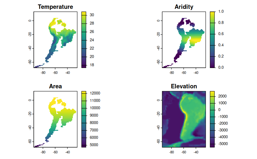
Nice. Now, we can create a input space using the create_spaces_raster function, just like in the previous vignette. We will use the withr package to save it in temporary directory, because we are only interested in the distance matrix.
The cost function we’ll use is simple: the cost will be defined by the Euclidean distance between source and destination cells, multiplied by a predefined coefficient. Note how this imply symmetry, because the distance between cell and cell is equal the other way around; i.e., . For the record, the Euclidean distance is defined as where is the longitude (x coordinate) and is the latitude (y coordinate).
Let’s get this going:
library(gen3sis2)

cf <- function(source, dest, cost_coef = 0.01) {
    euc_dist <- sqrt(((source$coordinates["x"] - dest$coordinates["x"])^2) + ((source$coordinates["y"] -
        dest$coordinates["y"])^2))
    cost = cost_coef * euc_dist

    return(cost)
}

raster_list <- list(temperature = temperature, aridity = aridity, area = area_r,
    elevation = elevation)

withr::with_tempdir({
    create_spaces_raster(raster_list = raster_list, cost_function = cf, directions = 8,
        output_directory = file.path(getwd(), "output"), full_dists = TRUE, overwrite_output = TRUE,
        verbose = FALSE, duration = list(from = 50, to = 0, by = -50, unit = "Ma"),
        geodynamic = TRUE, )
    files_created <- list.files(file.path(getwd(), "output"), recursive = T)

    distances_local <- readRDS(file.path(getwd(), "output", "distances_local", "distances_local_0.rds"))
})

distances_local
As our rasters had 5751 cells, our distance matrix is a 5751x5751 square matrix. Columns denote source cells, rows destination cells. Note, however, that not every cell is connected. We only computed the distances between a cell and its eight neighbors, using the direction argument. The symmetry of the matrix is pretty clear visually, with the main diagonal serving as a symmetry axis. For example, let’s call the cell 2000 as and cell 2071 as . is right above in the rasters. We can observe that going have the same cost as going , 1086.807.
Asymmetrical matrices
Now, consider that for some ecological reasons, the dispersal is influenced by the latitude. For example, going north is always harder than going south. To represent this, we will add a rule in the cost function (a if-else conditional): when direction is north, double the cost_coef.
We can achieve this latitudinal condition by comparing the coordinates of the cells. If the y coordinate of the destination cell is higher than the y coordinate of the source cell, it is going north:
cf <- function(source, dest, cost_coef = 0.01) {
    if (source$coordinates["y"] < dest$coordinates["y"]) {
        cost_coef <- 3 * cost_coef
    }

    euc_dist <- sqrt(((source$coordinates["x"] - dest$coordinates["x"])^2) + ((source$coordinates["y"] -
        dest$coordinates["y"])^2))
    cost = cost_coef * euc_dist

    return(cost)
}
In the cost function above, we tripled the cost_coef in case the destination is up north. Let’s see the impact of this in the distance matix:
withr::with_tempdir({
    create_spaces_raster(raster_list = raster_list, cost_function = cf, directions = 8,
        output_directory = file.path(getwd(), "output"), full_dists = TRUE, overwrite_output = TRUE,
        verbose = FALSE, duration = list(from = 50, to = 0, by = -50, unit = "Ma"),
        geodynamic = TRUE, )
    files_created <- list.files(file.path(getwd(), "output"), recursive = T)

    distances_local <- readRDS(file.path(getwd(), "output", "distances_local", "distances_local_0.rds"))
})

distances_local
The matrix still have the same format, however the values changed. For example, now going cost 3339.585 (going north), but going cost 1113.195 (going south). Moreover, the costs to move south, west and east remained the same, because we did not set any rule to these situation. In resume, the cost function controls it all.
Using external variables can make matrices more interesting
One common influential spatial aspect in this sense is the elevation. For example, often is more costly to disperse to higher than to lower elevations. In gen3sis2, these contexts when an external factor is relevant to dispersal can be easily modeled by asymmetrical matrices.
Let’s assume a context where elevation plays a major role in dispersal. In this, when species are moving up to higher places the resistance is greater than moving down, to lower places.
Now let’s implement a cost function that uses our “elevation” raster. In this the Euclidean distance will be multiplied by the elevation, and the final cost will be divided by :
cf <- function(source, dest) {

    euc_dist <- sqrt(((source$coordinates["x"] - dest$coordinates["x"])^2) + ((source$coordinates["y"] -
        dest$coordinates["y"])^2))

    cost <- abs(dest$value[["elevation"]]) * euc_dist

    return(cost/1e+06)
}

withr::with_tempdir({
    create_spaces_raster(raster_list = raster_list, cost_function = cf, directions = 8,
        output_directory = file.path(getwd(), "output"), full_dists = TRUE, overwrite_output = TRUE,
        verbose = FALSE, duration = list(from = 50, to = 0, by = -50, unit = "Ma"),
        geodynamic = TRUE, )
    files_created <- list.files(file.path(getwd(), "output"), recursive = T)

    distances_local <- readRDS(file.path(getwd(), "output", "distances_local", "distances_local_0.rds"))
})

distances_local
See that now going cost 565.503 and cost 564.389. Completely different.
Lastly, let’s imagine a scenario where elevation is greatly influential in species dispersal capabilities, but it is not relevant in the simulation itself. In this case, elevation could be added as an external argument in the cost function, as we saw before:
raster_list <- list(temperature = temperature, aridity = aridity, area = area_r)

cf <- function(source, dest, elev = elevation) {

    euc_dist <- sqrt(((source$coordinates["x"] - dest$coordinates["x"])^2) + ((source$coordinates["y"] -
        dest$coordinates["y"])^2))

    cost <- abs(terra::values(elev)[dest$index]) * euc_dist

    return(cost/1e+06)
}

withr::with_tempdir({
    create_spaces_raster(raster_list = raster_list, cost_function = cf, directions = 8,
        output_directory = file.path(getwd(), "output"), full_dists = TRUE, overwrite_output = TRUE,
        verbose = FALSE, duration = list(from = 50, to = 0, by = -50, unit = "Ma"),
        geodynamic = TRUE, )
    files_created <- list.files(file.path(getwd(), "output"), recursive = T)

    distances_local <- readRDS(file.path(getwd(), "output", "distances_local", "distances_local_0.rds"))
})

distances_local
Note how intricate and complex the matrix can get. Multiple factors can influence the dispersal and users can represented it using only the cost function.
Conclusion
This vignette provides a comprehensive guide to crafting highly customizable cost functions within the gen3sis2 framework. We’ve explored the fundamental anatomy of a cost function, emphasizing its adherence to R syntax, the requirement for a single numerical or Inf return value, and the mandatory source and dest arguments that provide detailed cell information.
A key takeaway is the profound impact of cost functions on distance matrix symmetry. By default, if no directional bias is encoded, gen3sis2 generates symmetrical matrices, where the cost of moving from A to B is identical to moving from B to A. However, we’ve demonstrated how incorporating conditional logic based on cell coordinates (e.g., latitude) or external environmental variables (e.g., elevation), for example, allows for the creation of asymmetrical matrices. This capability is valuable for accurately representing natural dispersal phenomena where movement might be easier or harder in specific directions. The ability to integrate external variables, even those not explicitly part of the primary raster input, further enhances the flexibility and ecological realism of dispersal simulations in gen3sis2.