6. Time in gen3sis2

1. Introduction

Eco-evolutionary processes take place across space and time. For this reason, time is also an important aspect of eco-evolutionary mechanistic models. There are many approaches to dealing with time (including constraints and rates) in ecology and evolution. In gen3sis2, time is particularly important when defining spaces and configuration files. In this vignette, we will see how to properly handle and make time explicit in gen3sis2 simulations.

2. Time in `gen3sis2`

2.1 Time and time units: what is accepted?

gen3sis2 is an interdisciplinary project that can be used as a tool across many fields. In addition, depending on the scope of the experiment and/or the organism being modeled, the simulation can operate on different time scales. This complexity, combined with the variety of ways time is measured across scientific disciplines, can sometimes make it difficult to compare experiments.

To promote standardization and reproducibility, gen3sis2 accepts only four time units: a (annum), ka (kilo-annum), Ma (mega-annum), and Ga (giga-annum). In addition to these, gen3sis2 also supports the flag-unit “timestep”, which will be explained later.

The choice of these four accepted time units is meant to strategically cover a wide range of possible temporal scales. Time in gen3sis2 is based on $a$ , which is equivalent to one year, and the remaining units are powers of ten of $a$ . See the table below:

time unit	a equivalent	power of ten
a	1 a	$10^0$ a
ka	1,000 a	$10^3$ a
Ma	1,000,000 a	$10^6$ a
Ga	1,000,000,000 a	$10^9$ a

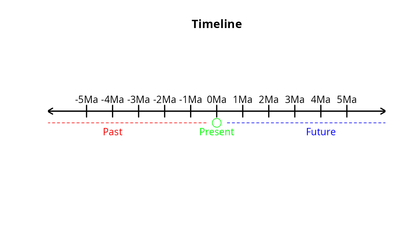
In gen3sis2, time is conceptualized as a number line. Negative values represent the past, zero represents the present, and positive values represent the future.

For example, if a simulation starts five million years ago and ends five million years in the future, we would say that it starts at $-5\text{Ma}$ and ends at $5\text{Ma}$ .

Visually, this situation can be represented by the following image:

2.2 Time and time-steps: how to deal with time in gen3sis_space_ objects

When creating your spaces, the function create_spaces_raster requires the duration parameter. This parameter must be provided as a list in the format list(from, to, by, unit).

The interpretation of the first two elements is straightforward: from defines when the environmental data starts, and to defines when it ends. The period between these two points in time is divided into equal intervals, known as time-steps. The by element of duration determines the length of each time-step, i.e., how much time is covered by each step, given the selected unit. Finally, unit specifies the time unit used (and therefore the time scale) and must be one of the accepted options: a, ka, Ma, or Ga.

This list format is intentionally similar to the base R function seq(from, to, by) and works in the same way.

The time-step is the backbone of a gen3sis2 simulation, because each process (dispersal, ecology, evolution, etc.) is simulated once per time step. In other words, the simulation is initialized at the first time-step and progresses sequentially until the last. Consequently, all metrics and simulation outputs are computed and reported based on these time-steps.

Users should be aware that the number of time-steps is an important modeling decision. For example, a simulation covering the period from −100 Ma to 0 Ma with 10 time steps of 10 Ma would run the processes 11 times. On the other hand, using 20 time steps of 5 Ma would result in 21 simulation steps. Therefore, these two simulations may not produce the same outcomes, especially when stochastic factors are involved.

Consider a space ranging from −5 Ma to 5 Ma (as described in the previous section), with each time step comprising 1 Ma. The corresponding function call would look like this:

create_spaces_raster(
  raster_list = your_environmental_rasters,
  cost_function = your_cost_function,
  output_directory = where_to_save_spaces.rds,
  duration = list(from = -5, to = 5, by = 1, unit = "Ma") # time is here
)

This will produce 11 time-steps:

2.3 Time and `step_time`: how to deal with time in config file

In the configuration file, time is defined using the variables step_time, start_time, and end_time.

The step_time variable sets the time scale at which the described processes take place. It must be provided as a list in the format list(x, unit), where unit is the chosen time unit and x is the numerical base.

For example, if step_time = list(x = 2.5, unit = "ka"), this means that the processes are designed to return the specified values every 2.5 ka (2,500 years). The relationship between this and the by element of the space duration will be discussed in the next section. The variables start_time and end_time define when the simulation should begin and end, respectively. These can be numeric values or NA.

The time unit must always remain consistent across the configuration. For example, if a simulation has step_time = list(x = 2.5, unit = "ka") and is intended to run from −10 ka to −2 ka, then the variables should be defined as start_time = -10 and end_time = -2. gen3sis2 will always assume that both start_time and end_time are expressed in the same unit as step_time.

If start_time = NA, the simulation will start at the earliest available time step. If end_time = NA, it will end at the latest available time step. If both are NA, the simulation will simply use all available time steps in the defined space.

2.4 Time and simulation: how the pieces fit together

To enhance reproducibility and allow experimentation with different configurations and spaces, gen3sis2 allows the use of configuration files and spaces that are not defined on the same time scale. For example, it is possible to use a configuration with step_time = list(x = 500, unit = "ka") together with a space constructed using duration = list(from = -10, to = 0, by = 1, unit = "Ma"). In this case, the space has time-steps spaced every 2 Ma, meaning that processes are simulated every 2 Ma, while the configuration assumes that processes occur every 1 Ma.

To reconcile these differences, when gen3sis2 reads the configuration file to initialize and run the simulation, it goes through a process of time interpretation. This process has two main objectives: (1) to understand how time is defined in both the configuration file and the space, and (2) to harmonize the time scales between them.

Not every process is time-dependent, but some are. Dispersal, for instance, usually depends on time, i.e., a species can disperse farther over longer periods. For dispersal, gen3sis2 automatically scales the returned values according to the time-step. For example, considering the configuration and space described above, if the dispersal value returned by the configuration is 500, the simulation assumes that this corresponds to each 1 Ma. Since each time step in the space spans 2 Ma, the value is automatically scaled to 1000 for each time-step. Similarly, isolated populations accumulate genetic divergence over time. Therefore, gen3sis2 also automatically scales the values obtained from the get_divergence_factor function.

The scaling process is fully transparent through on-screen messages and warnings. It is performed using a multiplier that indicates how many times an event should occur within each time-step. This multiplier is calculated as follows:

$scale\_time = \frac{conv\_unit \cdot S_t}{C_t}$ where

$S_t$ is the time-step of the space,
$C_t$ is the time-step of the config,
$conv\_unit$ is the conversion factor expressing one unit of the space’s time unit in the config’s time unit,
$step\_time$ is the resulting multiplier.

For example, consider the config and space described above, with step_time = list(x = 500, unit = "ka") and duration = list(from = -10, to = 0, by = 1, unit = "Ma"), respectively. In this case, $S_t = 1$ , $C_t = 500$ , and since $1\text{Ma} = 1000\text{ka}$ , $conv_unit = 1000$ . Therefore,

$scale\_time = \frac{1000 \cdot 1}{500} = 2$

This result indicates that config-defined events should occur twice per space time-step.

The multiplier is accessible to users through the joker variable scale_time, which is a simple numeric value available for any desired operation. For example:

get_dispersal_values <- function(n, species, space, config) {
  
  values <- rweibull(n, shape = 1.5, scale = 133)*scale_time # values will be properly scaled
  
  return(values)
}

Users should not define this variable within the config file, as it serves as a placeholder automatically replaced by config$user$scale_time during the simulation. Its sole purpose is to keep the code clean and concise. For instance, using config$user$scale_time instead of scale_time will produce the same result.

When gen3sis2 detects the use of scale_time inside any of the get_dispersal_values or get_divergence_factor functions, it automatically deactivates internal scaling for that process. This means that, if users prefer to handle time scaling manually (for example, using custom functions), they can simply include scale_time anywhere in their code:

get_dispersal_values <- function(n, species, space, config) {
  scale_time # no scaling will occur in this function
  
  values <- rweibull(n, shape = 1.5, scale = 133) 
  
  return(values)
}

For best-practice usage, it is recommended to call scale_time at the beginning of the function body.

If the user wishes to deactivate time scaling entirely, it is possible to set the config time unit to “timestep”. In this case, the config is always interpreted as being in the same temporal framework as the spaces. For example, using step_time = list(x = 1, unit = "timestep") completely disables time scaling. When “timestep” is used as the time unit:

The value of x becomes irrelevant and is ignored.
The scale_time multiplier is automatically set to 1.

This approach is useful when temporal consistency between config and spaces is already ensured, or when users prefer to work with abstract, step-based time rather than explicit chronological units.

2.5 Human and machine config

As said above, when the config file the used provided is read by gen3sis2 (in run_simuation() or create_input_config()), it goes trough a process of interpretation. In this processes, many aspects of the config are adapted to ensure that the simulation will run without problems. One central points is to replace the place-holder scale_time by the callable config$user$scale_time. In addition to that, code commentaries are removed, gen3sis2 detects whether the user used scale_time inside any of the main functions or not. Finally, the adapted code is parsed and evaluated.

The file provided by the user is called in gen3sis2 as “human config”. After this code is parsed and evaluated, it produces a list config that is stored internally during the simulation (and saved within the simulation state). This is called the “machine config”. They essentially carry the same information, but the machine config is interpreted, adapted and easily accessed by the simulation (and the user, when desired).

3. Conclusion

Time is an important aspect of eco-evolutionary simulations, and dealing with it in gen3sis2 is straight-forward. Every config file must be written considering time, as well as every space created. Config and space can have different timeframes, but in tis case gen3sis2 will calculate a multiplier and apply it to config’s processes, what can generate distortions.

14.04.2026