4. Plotting stuff

Introduction

Plotting in gen3sis2 is quite easy, as the package features several plotting functions to use in different contexts:

plot_space_overview
plot_space
plot_species_presence
plot_abundance
plot_richness

The core of plotting functions of gen3sis2 is built with ggplot2. Among other things, this allows for plots to be easily customizable. In this vignette, we will go through an overview of gen3sis2 plotting functions and how to customize your plot.

Visualizing the space

From your spaces.rds

If you inspect your spaces.rds file, you will see that it consists of an organized list of matrices and vectors, which aren’t too good for visualization. To better visualize the spaces created, users can use the plot_space_overview function, that will plot one or more variable for defined time-steps.

Let’s see an example:

library(gen3sis2)
# Load some spaces.rds create with create_spaces_raster...
space <- readRDS(system.file("extdata/SouthAmerica/space/spaces.rds", package = "gen3sis2"))

# ... and plot it!
# "env_names" selects the variables of interest
# "breaks" selects the timesteps of interest
plot_space_overview(space, env_names = "temp", breaks = c(-5, -2, 0))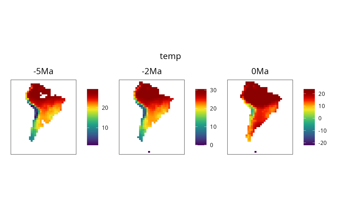

From inside the simulation (called in the config)

The observer function is a great place to make plot calls, and gen3sis2 features several functions to be called in this context. For example, it is possible to plot the space in the current time-step using the function plot_space.

As this vignette is for illustration purposes only, let’s define a function that will allow us to simulate how your space looks like inside the simulation:

simulate_space_format <- function(config,space,output_directory) {
  directories <- prepare_directories(config_file = config,
                                     input_directory = space,
                                     output_directory = output_directory)
  config <- create_input_config(config_file = config)
  config[["directories"]] <- directories
  val <- list("data" = list(),
              "vars" = list(),
              "config" = config)

  val$config <- gen3sis2:::complete_config(val$config)
  val$config$gen3sis$general$verbose <- 1
  val <- gen3sis2:::setup_inputs(val$config, val$data, val$vars)
  val <- gen3sis2:::setup_variables(val$config, val$data, val$vars)
  val <- gen3sis2:::setup_space(val$config, val$data, val$vars)
  return(val$data)
}

# 
config <- create_input_config(system.file("extdata/SouthAmerica/config/config_southamerica.R", package = "gen3sis2"))

data <- simulate_space_format(
  config = system.file("extdata/SouthAmerica/config/config_southamerica.R", package = "gen3sis2"),
  space = system.file("extdata/SouthAmerica/space", package = "gen3sis2"),
  output_directory = tempdir()
)

## config found:  /tmp/RtmpLdHDTk/temp_libpath3aa51f7235bc/gen3sis2/extdata/SouthAmerica/config/config_southamerica.Rspace found: /tmp/RtmpLdHDTk/temp_libpath3aa51f7235bc/gen3sis2/extdata/SouthAmerica/space 
## Output directory is: /tmp/Rtmpl22iSg/config_southamerica

names(data)

## [1] "inputs" "space"

[!] IMPORTANT: This is done only for this vignette, to facilitate the example.

Now, we can call the plot function in a very easy way:

plot_space(data$space)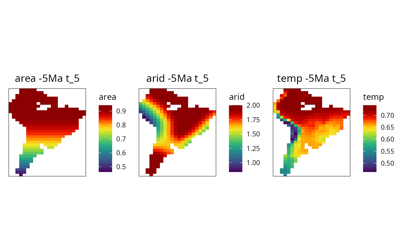

Again, this function is meant to be called inside the simulation and configured in the config file. plot_space_overview, however, is meant to be called outside the simulation, using the spaces.rds.

Visualizing species

Presence

The plot_species_presence is a useful function that users can use to plot the species’ presence across the space.

# Simulate species in random places
set.seed(13)
random_places <- sample(row.names(data$space$coordinates), 12)
sp <- gen3sis2::create_species(random_places, config)

# the same space we simulated before
plot_species_presence(sp, data$space)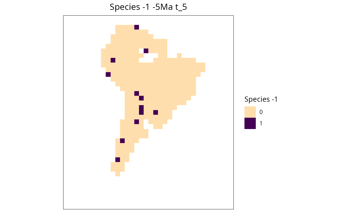

Abundance

# Simulate species in random places...
sp <- gen3sis2::create_species(random_places, config)

# ... and with random abundance
sp$abundance[] <- sample(1:5, 12, replace = TRUE)

# the same space we simulated before
plot_species_abundance(sp, data$space)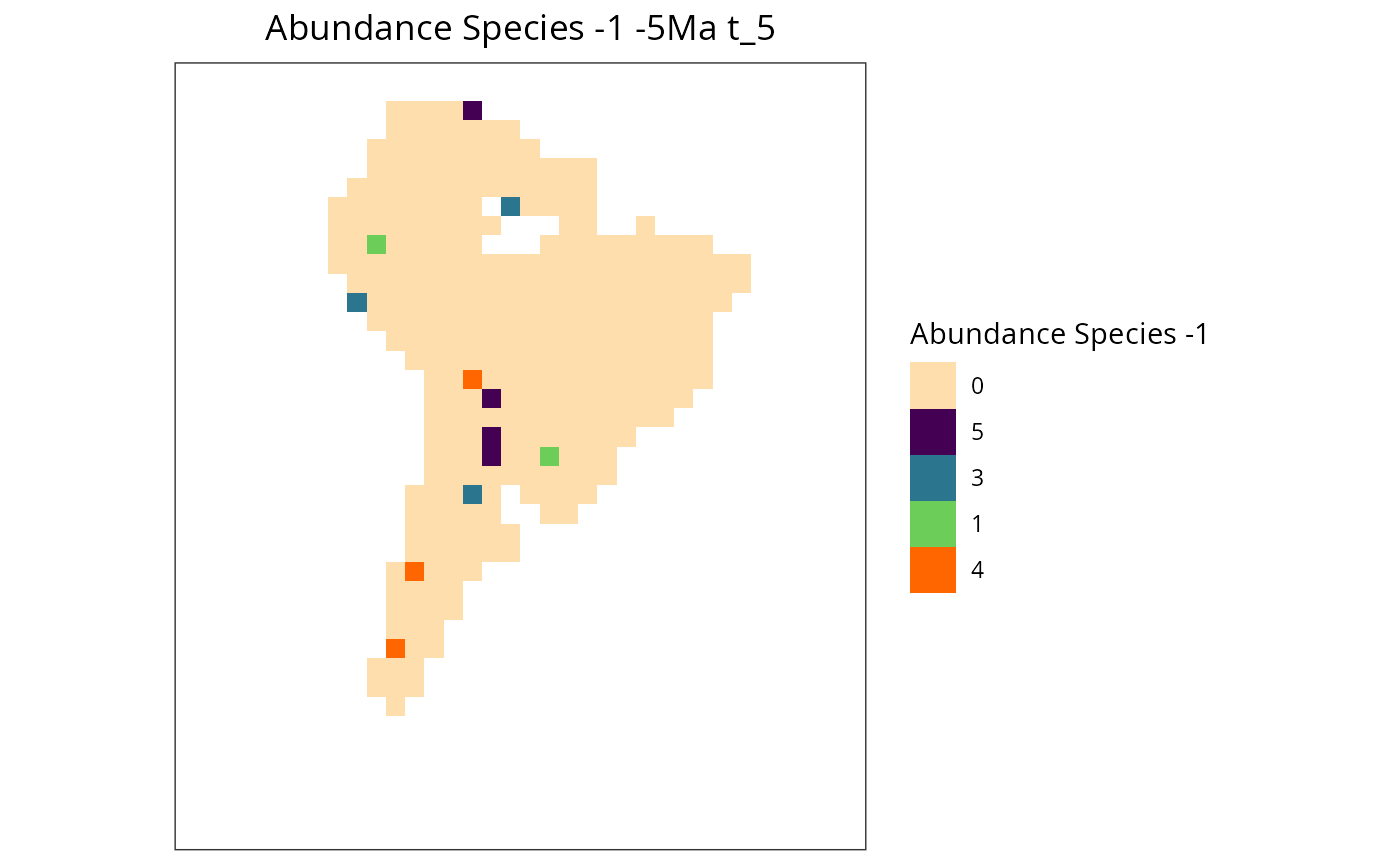

The scale of the plot is adaptive If the abundance vector of the species has few unique values, it creates a discrete scale. However, if the vector has a lot of unique values, it creates a continuous scale:

# Simulate species in random places...
sp <- gen3sis2::create_species(random_places, config)

# ... and with random abundance
sp$abundance[] <- sample(1:200, 12, replace = TRUE)

# the same space we simulated before
plot_species_abundance(sp, data$space)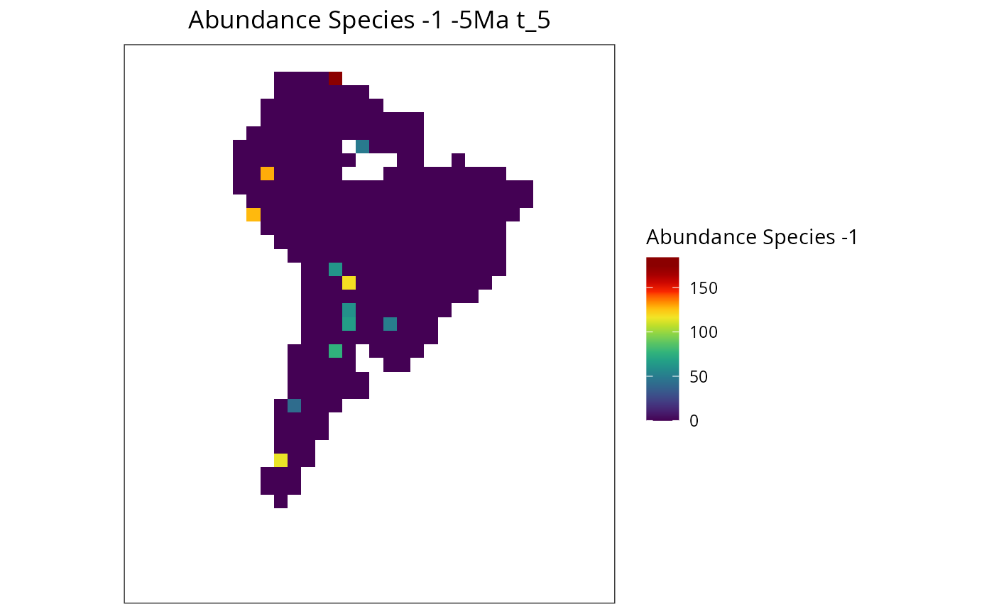

Richness

Species richness across the space is very useful information for users. For that reason, gen3sis2 features the plot_richness function, which can be used within the config to plot species richness. Different from the other functions, this one will receive a species list, not a single species. But, besides that, it works in the very same way:

# Simulating a species list
## inside the simulation this will be called "all_species"
species_list <- list(
  gen3sis2::create_species(random_places[1:10], config),
  gen3sis2::create_species(random_places[5:10], config),
  gen3sis2::create_species(random_places[8:12], config)
)

plot_richness(species_list, data$space)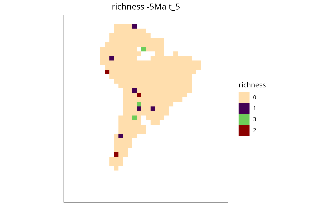

Plot aesthetics customization

Many aspects of the plot can be customized, ranging from simple to complex custom settings. This is possible due to the plotting core being built with ggplot2. Let’s see some possibilities.

Customizing color

The simplest way to customize plots is by defining colors, using the col parameter. Each context has its specifications, so the user needs to read functions’ documentation to be aware of the proper usage. However, let’s go over one simple example:

# Simulate species in random places
set.seed(13)
random_places <- sample(row.names(data$space$coordinates), 12)
sp <- gen3sis2::create_species(random_places, config)

# It is possible to set any color, using names or hex codes
plot_species_presence(sp, data$space, col = c("lightgray","#8B0000"))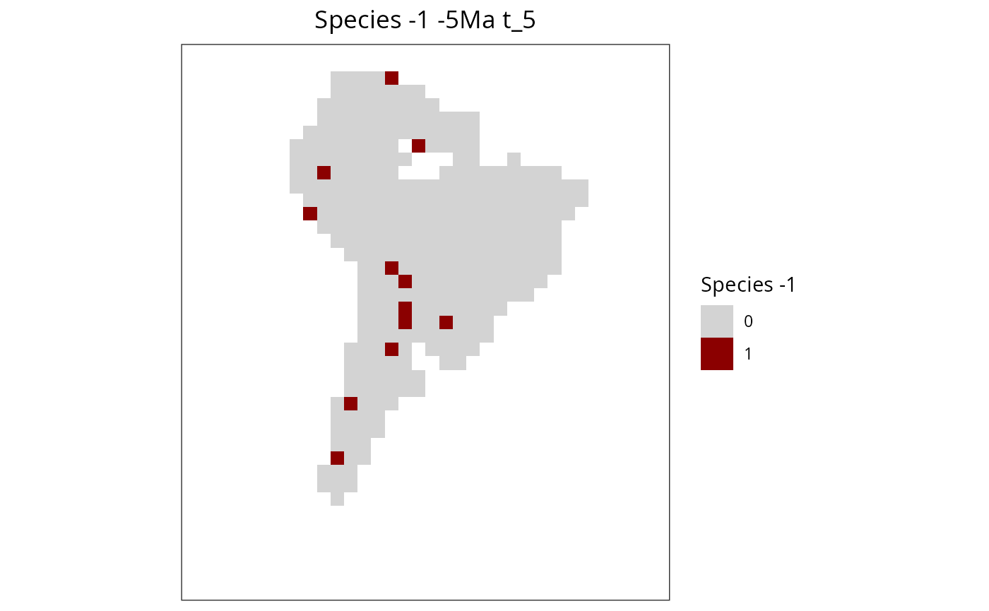

Applying `ggplot2` syntax

As the plotting core of gen3sis2 is the ggplot2 package, plotting functions return ggplot2 objects. As a result, it’s natively possible to apply ggplot2 syntax gen3sis2 plots:

# storing plot in an object 
p <- plot_species_presence(sp, data$space, col = c("black","#1B8200"))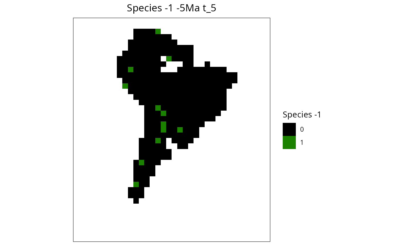

# applying ggplot2 syntax
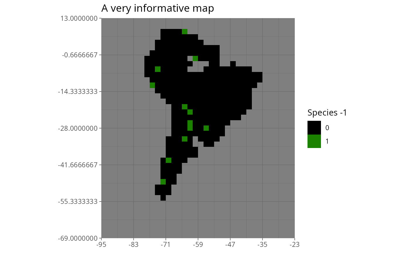
p +
  ggplot2::theme_dark() +
  ggplot2::labs(
    title = "A very informative map"
  )

Customizing `gen3sis2` default aesthetics

Default plot aesthetics in gen3sis2 are stored as internal functions .default_raster_plot_aesthetics, for raster type spaces, and .default_sf_plot_aesthetics, for h3 and points type spaces. This allows users to customize the aesthetics from all plots in the session, by overriding package’s options:

First, let’s see how the default raster aesthetics look:

gen3sis2:::.default_raster_plot_aesthetics

## function (space, col, x_breaks, y_breaks, title) 
## {
##     list(ggplot2::scale_x_continuous(expand = c(0, 0), breaks = x_breaks), 
##         ggplot2::scale_y_continuous(expand = c(0, 0), breaks = y_breaks), 
##         ggplot2::theme_bw(), ggplot2::theme(plot.title = ggplot2::element_text(hjust = 0.5), 
##             panel.grid.major = ggplot2::element_blank(), panel.grid.minor = ggplot2::element_blank(), 
##             axis.text = element_blank(), axis.ticks = element_blank()), 
##         ggplot2::labs(title = title), ggplot2::coord_fixed(ratio = 1))
## }
## <bytecode: 0x6540f0d3de30>
## <environment: namespace:gen3sis2>

Now, let’s override it, defining our own aesthetics:

library(scales)
options(gen3sis2.raster_plot_aesthetics = function(space, col, x_breaks, y_breaks, title) {
  list(
    ggplot2::scale_x_continuous(
      expand = c(0, 0),
      breaks = x_breaks,
      labels = function(x) round(x, 0) # changed x axis labels...
    ),
    ggplot2::scale_y_continuous(
      expand = c(0, 0),
      breaks = y_breaks,
      labels = function(y) round(y, 0) # and y labels...
    ),
    ggplot2::theme_dark(), # and the theme...
    ggplot2::theme(
      plot.title = ggplot2::element_text(hjust = 0.5),
      panel.grid.major = ggplot2::element_line(color = alpha("white", 0.5), linewidth = 0.2), # and background lines...
      panel.grid.minor = ggplot2::element_line(color = alpha("white", 0.4), linewidth = 0.1),
      axis.text = ggplot2::element_text()
    ),
    ggplot2::labs(title = "Look, mom. It's custom!"), # and title.
    ggplot2::coord_fixed(ratio = 1) # To freeze the map ratio.
  )
})

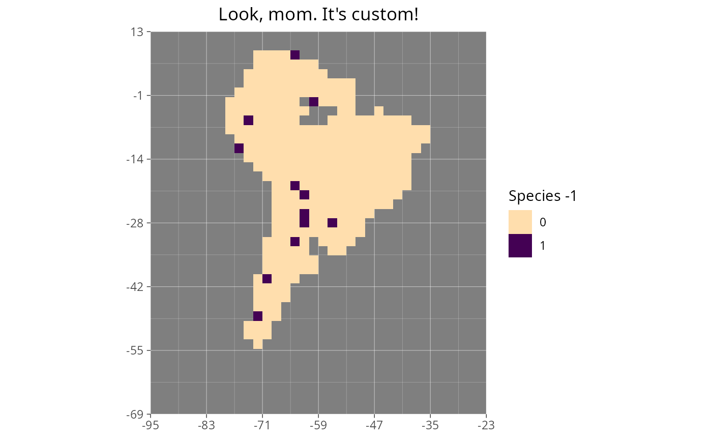
Now the plots should have this new aesthetics:

plot_species_presence(sp, data$space)

14.04.2026