
gen3sis: general engine for eco-evolutionary simulations
In this vignette you will be introduced to gen3sis, an engine for simulating various spatial eco-evolutionary models. Here we will create a virtual planet, populate it and implement evolution, then examine our virtual species.
In particular, we will go through the following steps:
1. Set-up the input files needed by the gen3sis package, specifically the space objects, which defines the spatial confines of the simulation, and the configuration file, which defines the parameters used.
2. Run a simulation.
3. Visualise the outputs.
4. Analyse the outputs.
We will do this using a highly simplified example. Here we will model the evolution of species in South America over the last five million years.
First of all, we will load the packages we need, including the gen3sis package.
If you run into problems, you can refer to the full help documentation in gen3sis.
Let’s check the version of the gen3sis package we are using.
# Print the version of the package being used
packageVersion("gen3sis2")
#> [1] '1.0.0'
1. Set-up
Before we can run a gen3sis simulation, we need to generate files containing the input data and model settings. For this example, we have provided environmental data for South American over the Cenozoic. To access this dataset, we will define the path to the data contained inside the package.
# Set the filepath to the location in gen3sis2 files with test data
datapath <- system.file(file.path("extdata", "SouthAmerica"), package = "gen3sis2")

# View contents of SouthAmerica folder
list.files(datapath, recursive = TRUE)
#>  [1] "config/config_southamerica_observer.R"
#>  [2] "config/config_southamerica.R"
#>  [3] "images/const_cost.png"
#>  [4] "images/introduction_richness.png"
#>  [5] "images/v2varplot.png"
#>  [6] "images/var_cost.png"
#>  [7] "input_rasters/area_rasters.grd"
#>  [8] "input_rasters/area_rasters.gri"
#>  [9] "input_rasters/aridity_rasters.grd"
#> [10] "input_rasters/aridity_rasters.gri"
#> [11] "input_rasters/temperature_rasters.grd"
#> [12] "input_rasters/temperature_rasters.gri"
#> [13] "output/sgen3sis.rds"
#> [14] "space/distances_local/distances_local_0.rds"
#> [15] "space/distances_local/distances_local_1.rds"
#> [16] "space/distances_local/distances_local_2.rds"
#> [17] "space/distances_local/distances_local_3.rds"
#> [18] "space/distances_local/distances_local_4.rds"
#> [19] "space/distances_local/distances_local_5.rds"
#> [20] "space/METADATA.txt"
#> [21] "space/spaces.rds"
#> [22] "species_and_spaces/space_t_2.rds"
#> [23] "species_and_spaces/species_t_2.rds"
Ultimately, our experiment folder should look like this:
| >EXPERIMENT_FOLDER |
|---|
| >space |
| >distances_local |
| >spaces.rds |
| >METADATA.txt |
| >config |
| >config.R |
We will start by preparing the contents of the space
folder, followed by the config file.
1a. Space
Our first task is to create the spatial objects ready to input into gen3sis. These objects are:
a
spaces.rdsfile, containing (i) the geographic coordinates of the space cells, (ii) corresponding information on which cells can be occupied by the organisms modeled (e.g. land or ocean), and (iii) the environmental conditions relevant to the species’ ecology;a series of
.rdsfiles, one for each time-step, describing distance matrices between the sites.
We will generate these using the create_spaces_raster()
function.
Loading the environmental data
Our first step is to load raster files containing the spatio-temporal
distributions of our environmental variables of interest. Here, we will
use temperature, aridity and cell area rasters for South America. Each
raster comes in two components, a .grd file and a
.gri file.
# View contents of input raster folder
list.files(file.path(datapath, "input_rasters"))
#> [1] "area_rasters.grd"        "area_rasters.gri"
#> [3] "aridity_rasters.grd"     "aridity_rasters.gri"
#> [5] "temperature_rasters.grd" "temperature_rasters.gri"
We will load the three data files from the example data and convert each of them into a SpatRaster.
# Create a SpatRaster of the temperature change through time
temperature_raster <- rast(file.path(datapath, "input_rasters/temperature_rasters.grd"))
temperature_raster <- temperature_raster[[order(names(temperature_raster), decreasing = T)]]
# Create a SpatRaster of the aridity change through time
aridity_raster <- rast(file.path(datapath, "input_rasters/aridity_rasters.grd"))
aridity_raster <- aridity_raster[[order(names(aridity_raster), decreasing = T)]]
# Create a SpatRaster of the cell area (static in time)
area_raster <- rast(file.path(datapath, "input_rasters/area_rasters.grd"))
area_raster <- area_raster[[order(names(area_raster), decreasing = T)]]
# make sure that they are ordered from past to present
We will now generate a list containing all of the environmental data, with each variable named. It is also possible to create a list using the raster file paths on your hard drive, instead of loading all the data into R.
# Create a list with three elements, each named and corresponding to a raster
spaces_list <- list(temp = temperature_raster, arid = aridity_raster, area = area_raster)
Setting up the distance matrix
The second step is to determine the distances between our sites, which we will do by defining a cost function. Essentially we are defining the species’ dispersal ability, and therefore whether dispersal between each pair of sites is feasible or not.
First, we will look at a simple case, in which the migration cost is equal to the distance between sites in grid cell units, multiplied by the raster resolution. For landscapes with a coordinate system (crs), the cost is defined in meters: by dividing the cost function by 1000, we get the cost of travelling 1 km.
We can define a simple cost function in which dispersal is not penalised:
# Define simple cost function, with cost given in kilometers
cost_function_null <- function(source, habitable_src, dest, habitable_dest) {
    return(1/1000)
}
We can now generate our spaces.rds file and distance
matrices by inputting our environmental data and cost function into the
create_spaces_raster() function. Before we do that, there
are a few other parameters required by the function that we need to
choose values for.
The argument directions sets the number of neighbouring
directions in which to determine connectivity, and can take the values
4, 8, or 16. For this example, we will use 8 directions.
The argument full_dists defines whether one large
distance matrix is created for all suitable sites (TRUE) or a list of
small distance matrices is generated for the neighboring sites specified
in ‘directions’ around each suitable site (default; FALSE). The full
distance matrix confers faster computing speed for the model, but
requires larger storage.
The argument duration is where we define the time-steps
used in the spaces objects.
The crs argument can also be used to set the geographic
coordinate system, allowing for global spherical distance correction.
Here we are using the world geodetic system (WGS84).
Finally, the geodynamic argument informs the function of
whether the environmental rasters (including cell area) change through
time. We have one raster for each 1My of our simulation, so we set this
value to TRUE.
Finally, do not forget to specify/describe the space data you just created. We recommend storing it in form of a METADATA.txt file within the spaces folder.
We have now generated our necessary spaces objects based on our empirical environmental data. Alternatively, if you want to see an example of how you can create a virtual dynamic space from scratch, please refer to the design_landscape vignette.
Alternatively, you can load our pre-made spaces
object.
Here our spaces object contains temperature and aridity
values. We can access the spaces.rds object, and create
maps of our environmental conditions.
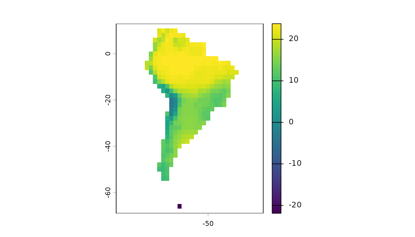
This figure shows the temperature and aridity of the space used in this vignette at 5 and 0Ma.
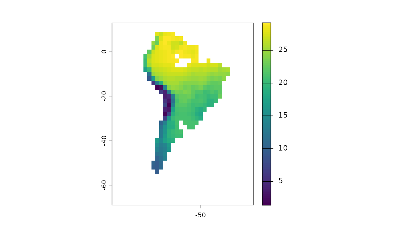
This figure shows the temperature and aridity of the space used in this vignette at 5 and 0Ma.
The second space class defines the permeability of the space for species movement between cells via dispersal. The connection cost between sites is computed for each time step from the gridded space data based on haversine geographic distances modified by a user-defined cost function. Distance matrices containing the connection costs are provided at every time step, as either: (i) a pre-computed full distance matrix, containing all habitable cells in the space (faster simulations but more storage required); or (ii) a local distance matrix, computed from neighboring site distances up to a user-defined range limit (slower simulations but less storage required).
We can see these already generated in our
space/distances_local repository, with one matrix for each
time step.
#> [1] "distances_local_0.rds" "distances_local_1.rds" "distances_local_2.rds"
#> [4] "distances_local_3.rds" "distances_local_4.rds" "distances_local_5.rds"
1b. Configuration
The configuration object defines the core processes of the system modeled, formalising eco-evolutionary processes and defining run settings.
The core functions include custom initialization, observer, speciation, dispersal, evolution and ecology functions. Altogether, these six functions are applied as defined in the simulation engine. The possibility to customise these functions confers the high flexibility and generality of gen3sis in terms of including a wide range of theoretical knowledge.
Additional settings include the ecological traits considered in the simulation; whether a random seed is used thus enabling simulation reproducibility; start and end times of the simulation; and rules about aborting the simulation, including the maximum global or local species number permitted.
For this example, we will generate an empty config file, populate it, and show how it can also be edited.
First, to create an empty config, we will use the function write_config_skeleton, defining the output location and file name.
# Write config skeleton in specified folder
write_config_skeleton("/Choose/your/directory/SouthAmericanConfig.R")
If successful, TRUE will be printed here.
We can now open our skeleton file and start populating it.
We will briefly explore the different components of the configuration file, entering values and modifying where needed to produce a simple model set-up.
Metadata
The first section contains metadata, such as when and by whom the file has been created, and which spaces object it was made for. It can also include information about intentions of the specific configuration, and any associated publications. This information is designed to be human-readable.
# Enter your name as the author of the configuration file.

# For `space`, we will enter the geographic extent: South America.

# For `Description`, give a brief outline of the model remit and your goals in
# running this gen3sis model.
General settings
Here we are able to set various overarching settings for the model. We can see the option to set a random seed, and set temporal, environmental and biodiversity constraints on the simulation.
We will leave most of these values at the default - for the temporal settings, this means that these values will be inherited from our spaces object.
However, we will alter the traits modeled in our simulation, set using traits_names. In addition to the default dispersal ability possessed by our species, we also want them to have optimum temperature traits.
We also need to normalise the environmental values. We will do this
by providing a list of the raster objects to
environmental_ranges, each given the value NA.
This will scale each between 0 and 1, based on the minimum and maximum
values present in the dataset.
Observer
The observer function is how the virtual world is recorded, defining the outputs that are saved at specified time steps. Results can also be exported and plotted in real time, as the model runs. No settings are provided as defaults here, but a list of example outputs are given in the notes provided.
Here we will save the species richness, and generate plots in real time, which are also saved inside the plot folder.
# Modify
end_of_timestep_observer = function(data, vars, config) {
}
# to
end_of_timestep_observer = function(data, vars, config) {
    save_species()
}
Initialization
The initialization function creates the ancestral species present at
the start of the simulation, using the function
create_ancestor_species(). Users can define the number of
ancestors, their distribution across the palaeolandscape, and their
trait values.
In our example, we will generate an initial 10 ancestor species, each of which is randomly inhabiting one site. We will restrict the region of colonization to South America by limiting the range to a spatial extent of c(-95, -24, -68, 13). All sites have an equal probability of being inhabited by a species in the beginning of the simulation.
We will set the optimum temperature trait, temp, of each initial species population to the temperature of its site, meaning it is adapted to the local conditions. We will set all ancestral dispersal traits to 1.
# Retain
initial_abundance = 1

# Modify
create_ancestor_species <- function(space, config) {
    stop("create the initial species here")
}
# to
create_ancestor_species <- function(space, config) {
    range <- c(-95, -24, -68, 13)
    co <- space$coordinates
    selection <- co[, "x"] >= range[1] & co[, "x"] <= range[2] & co[, "y"] >= range[3] &
        co[, "y"] <= range[4]
    new_species <- list()
    for (i in 1:10) {
        initial_cells <- rownames(co)[selection]
        initial_cells <- sample(initial_cells, 1)
        new_species[[i]] <- create_species(initial_cells, config)
        new_species[[i]]$traits[, "temp"] <- space$environment[initial_cells, "temp"]
        new_species[[i]]$traits[, "dispersal"] <- 1
    }
    return(new_species)
}
Core Processes
Dispersal
The dispersal function determines, for each species population, the connectivity between sites and the colonization of new sites.
In our example, species dispersal between time-steps is stochastic and follows a Weibull distribution. This distribution can easily be right-skewed, allowing for infrequent long-distance dispersal events. This distribution is consistent between species.
# Generate a histogram illustrating the Weibull distribution
hist(rweibull(1000, shape = 1.5, scale = 133), main = NA, xlab = "Value", col = "black")
Speciation
The speciation function iterates over each existing species, registers its range, and determines when geographic isolation between population clusters is higher than a user-defined threshold, triggering a lineage splitting event (cladogenesis).
In our example, we will set speciation to take place after 2 time-steps of isolation. Since our space consists of 1 My time-steps, this corresponds to 2 My of isolation needed for species divergence.
# Modify
divergence_threshold = NULL
# to
divergence_threshold = 2
Using get_divergence_factor, we will indicate that the divergence increase is the same for all species.
Trait evolution
In the trait evolution function, clustered populations (those which can exchange genes) have their trait values summarised. Trait value averaging is weighted by abundance, meaning that the most common trait values will have more influence over the perceived average. After this, mutation of the trait value occurs, based on a normal distribution with standard deviation of 0.001. Here we are only manipulating the “temp” trait, meaning that the optimum temperature value of each population is calculated, then mutated, allowing this value to increase or decrease.
# Modify
apply_trait_evolution <- function(species, cluster_indices, space, config) {
    stop("mutate species traits here")
}
# to
apply_trait_evolution <- function(species, cluster_indices, space, config) {
    trait_evolutionary_power <- 0.001
    traits <- species[["traits"]]
    cells <- rownames(traits)
    for (cluster_index in unique(cluster_indices)) {
        cells_cluster <- cells[which(cluster_indices == cluster_index)]
        mean_abd <- mean(species$abundance[cells_cluster])
        weight_abd <- species$abundance[cells_cluster]/mean_abd
        traits[cells_cluster, "temp"] <- mean(traits[cells_cluster, "temp"] * weight_abd)
    }
    mutation_deltas <- rnorm(length(traits[, "temp"]), mean = 0, sd = trait_evolutionary_power)
    traits[, "temp"] <- traits[, "temp"] + mutation_deltas
    return(traits)
}
Ecology: Biotic and Abiotic Interactions
The ecology function determines the presence, and abundance, of the populations in occupied sites. Species populations are updated the basis of local environmental values, updated co-occurrence patterns, and species traits.
In our example, we will calculate abundances based on how close the population’s optimum temperature value is to the site temperature. We scale the values to avoid small numbers and apply a carrying capacity based on aridity and temperature corrected by the area of a site. If abundances are below 1, species are considered extinct, if total abundance in a site is above the carrying capacity, small abundances are removed progressively and randomly distributed across the present species until total abundance is smaller or equal to the carrying capacity.
# Modify
apply_ecology <- function(abundance, traits, local_environment, config) {
    stop("calculate species abundances and deaths here")
}
# to
apply_ecology <- function(abundance, traits, local_environment, config) {
    abundance_scale = 10
    abundance_threshold = 1
    survive <- abundance >= abundance_threshold
    abundance[!survive] <- 0
    abundance <- ((1 - abs(traits[, "temp"] - local_environment[, "temp"])) * abundance_scale) *
        as.numeric(survive)
    abundance[abundance < abundance_threshold] <- 0
    k <- ((local_environment[, "area"] * (local_environment[, "arid"] + 0.1) * (local_environment[,
        "temp"] + 0.1)) * abundance_scale^2)
    total_ab <- sum(abundance)
    subtract <- total_ab - k
    if (subtract > 0) {
        while (total_ab > k) {
            alive <- abundance > 0
            loose <- sample(1:length(abundance[alive]), 1)
            abundance[alive][loose] <- abundance[alive][loose] - 1
            total_ab <- sum(abundance)
        }
        abundance[!alive] <- 0
    }
    return(abundance)
}
It is also possible to set up Biotic Modification of the Environment, but in this example we will not include this and leave the values to default.
Before using your config, you can test whether it is valid. If the function verify_config returns TRUE, you are good to go.
# Check whether config settings conform to *gen3sis* requirements
verify_config(config_object)
Alternatively, we already have this configuration file prepared, which we can view.
2. Run
Now that we have set up our input files, we can run a simulation using the run_simulation function. This function will:
Read in the config and initial space, and call create_ancestor_species from the user config to create the initial species distributions for the simulation.
Loop over the time-steps. For every time-step the appropriate space is loaded, and eco-evolutionary processes are implemented.
At the end of every time-step, the simulation saves the species, landscapes, species richness patterns, etc… by calling the end_of_timestep_observer from the user config.
When the simulation reaches the end, a summary of requested outputs is saved in the output folder.
To launch a simulation you need to call the run_simulation
function. For simplicity, here we will only store one intermediate step
between the starting and end time-steps by setting
call_observer = 1. We will also set
verbose = 0 to minimise printed outputs for such a simple
simulation, but more information can be provided if desired.
# Run the simulation
sim <- run_simulation(config = file.path(datapath, "config/config_southamerica.R"),
    space = file.path(datapath, "space"), output_directory = tempdir(), call_observer = 1,
    verbose = 0)
Additionally to the main functions, gen3sis provides several convenience functions to generate input data, configuration files, and plots. Moreover, all functions are accessible to the observer functions, which requests the variables for logging and calculation during the model runs. This allows the output of the simulation to be stored in a format that can be readily analysed. Here, our config set-up has produced plots of species richness at our starting (5Ma), single observer call (3Ma) and final (0Ma) time steps.
After the simulation is finished, output files are automatically stored in a sub-folder called output.
3. Visualise
gen3sis returns a summary object (of
gen3sis_output class) at the end of the simulation, storing
default summary statistics and important data over time. Here we stored
the summary object as sim, as well as saving it to the
output folder.
We can quickly visualise some main results using the
plot_summary() function.
# Plot main summary statistics
plot_summary(sim)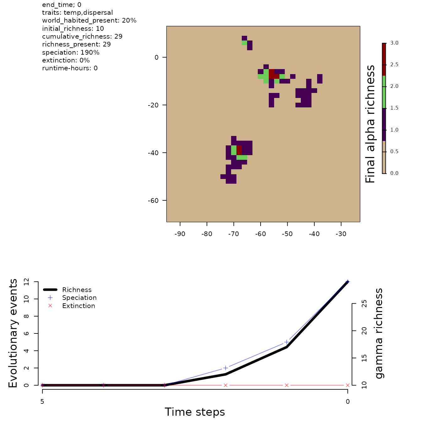
There are a few visualization tools already included in the package, but you are free to explore and check the outputs with your favourite plotting functions and colors.
4. Analyse
We are now ready to perform analyses to investigate the model’s behaviour. Typically this will be the way in which we determine how our simulation relates to the hypothesis we are trying to test. Here, we set a lower limit on total abundance in colder and more arid environments, so we expect that the number of species that can co-exist also decreases in those environments: we can now investigate that in more detail.
Before we perform a few statistical analyses, we first need to
combine environmental data from our spaces object with the
simulated species richness in the sim output object.
# Bind together environmental variables at time step 0
space_t0 <- as.data.frame(cbind(spaces$env$temp[, 1:2], temp = spaces$env$temp[,
    3], arid = spaces$env$arid[, 3], area = spaces$env$area[, 3]))
# Add species richness to the dataframe
space_t0 <- cbind(space_t0, rich = sim$summary$`richness-final`[, 3])
# Remove NAs
space_t0 <- na.omit(space_t0)
Now we want to investigate the relationship between species richness and our environmental variables at the final time-step of the simulation.
First, we can fit a generalised linear model between richness and temperature.
# Fit generalised linear model
glm.uni <- glm(rich ~ poly(temp, 2), data = space_t0, family = poisson)
# Print correlation between temperature and richness
cor(space_t0$temp, space_t0$rich)
#> [1] -0.08121768
Now we can plot the response curve.
# Prepare temperature and richness data from our model
data_plot <- data.frame(cbind(space_t0$temp, predict(glm.uni, type = "response")))

# Sort data for plotting and omit NAs
data_plot <- na.omit(data_plot[order(data_plot[, 1], decreasing = FALSE), ])

# Get number of observations
n <- paste0("observations (n = ", length(space_t0$rich), ")")

# Plot model curve
plot(data_plot[, 1], data_plot[, 2], xlab = "Temperature [°C]", ylab = expression(paste(alpha,
    " richness")), frame.plot = F, type = "l", col = "red", lwd = 2, xlim = c(min(space_t0$temp),
    max(space_t0$temp)), ylim = c(min(space_t0$rich), max(space_t0$rich)))

# Add observed points
points(space_t0$temp, space_t0$rich, col = rgb(0.5, 0.5, 0.5, alpha = 0.4), pch = 16)

# Add legend
legend(-20, 30, col = c(rgb(0.5, 0.5, 0.5, 0.4), "red"), legend = c(n, "model fit"),
    pch = c(16, NA), lty = c(NA, 1), lwd = c(NA, 2), bty = "n")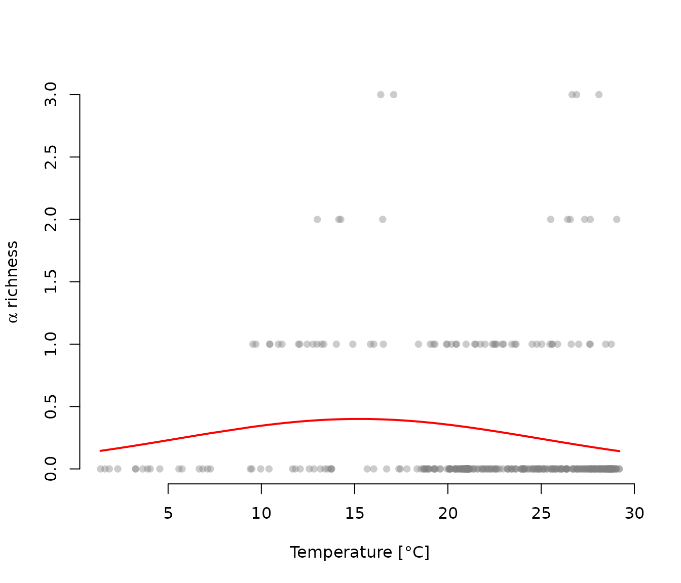
We can see that the relationship between the two variables is hump-shaped, indicating that species richness is highest at intermediate temperatures. The higher richness found above 10° is consistent with the ecological rule that we imposed: at higher temperatures, there is higher energy availability and capacity for species to coexist.
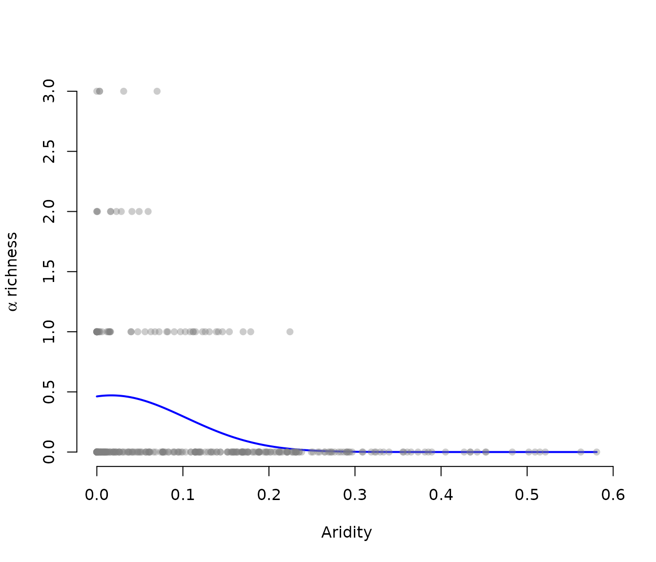
We observe a large spread in the points at higher temperatures. This is likely because high temperature regions frequently also have high aridity. Thus, we will next investigate the relationship between aridity and species richness by fitting another generalised linear model.
The number of species is negatively correlated with aridity. The explained deviance of this relationship is D2 = 0.202. This relationship emerges because we set a lower carrying capacity in cells with higher levels of aridity. Hence, the model behaves as expected relative to our configuration.
We can see this in more detail by plotting the curve.
It is important to consider that we have only been analysing the species richness at one time-step, namely the last one (0 Myr). The emerging patterns are likely not only influenced by the environmental conditions of the present, but also by historical conditions, as well as the complex process interactions enacted by gen3sis.
For more details on how to set up more complex or theoretical analyses, see our other vignettes. It’s now up to you to explore the “virtual” world.